2. Stereo-seq Hemibrian
Here, we analyzed the mouse brain data generated from Stereo-seq, including cortical regions, hippocampal regions, midbrain regions, thalamic regions, and fiber tracts. Raw data are avaiable at https://db.cngb.org/stomics/mosta/.
load data
[1]:
import  os
import warnings
warnings.filterwarnings('ignore')

import SECE
import torch
import numpy as np
import scanpy as sc

result_path = 'brain'
os.makedirs(result_path, exist_ok=True)
[2]:
adata = sc.read('./data/brain.h5ad')
sc.pp.filter_genes(adata, min_cells=20)
adata
[2]:
AnnData object with n_obs × n_vars = 50140 × 18575
    obs: 'annotation', 'x', 'y'
    var: 'n_cells'
    obsm: 'spatial'
    layers: 'counts'
Creating and training the model
[3]:
sece = SECE.SECE_model(adata.copy(),
                       likelihood='zinb',
                       result_path=result_path,
                       dropout_rate=0.1,
                       dropout_gat_rate=0.2,
                       device='cuda:1')
Likelihood: zinb
Input dim: 18575
Latent Dir: 32
Model1 dropout: 0.1
Model2 dropout: 0.2
[4]:
sece.adata.X.toarray() # Count matrix
[4]:
array([[0., 0., 0., ..., 0., 0., 0.],
       [0., 0., 0., ..., 0., 0., 0.],
       [0., 0., 0., ..., 0., 0., 0.],
       ...,
       [0., 0., 0., ..., 0., 0., 0.],
       [0., 0., 0., ..., 0., 0., 0.],
       [0., 0., 0., ..., 0., 0., 0.]], dtype=float32)
AE Module of SECE
[5]:
# Prepare input data for AE module
sece.prepare_data(lib_size='explog', normalize=True, scale=False)
Library size: explog
Input normalize: True
Input scale: False
Hvg: False
(50140, 18575)
[6]:
# train and predict for AE module
sece.train_model1(epoch1=50, plot=True)
adata1 = sece.predict_model1()
100%|████████████████████████████████████████████████████████████████████████████████████████████████████████████████████████████████████████████| 50/50 [29:19<00:00, 35.18s/it]
Model1 lr: 0.001
Model1 epoch: 50
Model1 batch_size: 128
GAT Module of SECE
[7]:
# Prepare input data for GAT module
sece.prepare_graph(cord_keys=['x','y'],
                   latent_key = 'X_CE',
                   num_batch_x=3,
                   num_batch_y=2,
                   neigh_cal='knn',
                   n_neigh=10,
                   kernal_thresh=0.5)
Batch 1: Each cell have 10.0 neighbors
Batch 1: Each cell have 43similar cells
Batch 2: Each cell have 10.0 neighbors
Batch 2: Each cell have 72similar cells
Batch 3: Each cell have 10.0 neighbors
Batch 3: Each cell have 61similar cells
Batch 4: Each cell have 10.0 neighbors
Batch 4: Each cell have 58similar cells
Batch 5: Each cell have 10.0 neighbors
Batch 5: Each cell have 73similar cells
Batch 6: Each cell have 10.0 neighbors
Batch 6: Each cell have 43similar cells
All: Each cell have 10.0 neighbors
Graph cal: knn
knn: 10
kernal_thresh: 0.5
[8]:
# train and predict for GAT module
sece.train_model2(  lr_gat=0.01,
                    weight_decay_gat=0,
                    epoch2=40,
                    re_weight=1,
                    si_weight=0.08,
                    plot=True)
adata1 = sece.predict_model2()
100%|████████████████████████████████████████████████████████████████████████████████████████████████████████████████████████████████████████████| 40/40 [00:44<00:00, 1.11s/it]
Model2 lr: 0.01
Model2 epoch: 40
Model2 similar weight: 0.08
[9]:
adata1
[9]:
AnnData object with n_obs × n_vars = 50140 × 18575
    obs: 'annotation', 'x', 'y', 'size', 'n_counts'
    var: 'n_cells'
    uns: 'log1p'
    obsm: 'spatial', 'X_CE', 'X_SE'
    layers: 'counts', 'expr'
Clustering
Clustering for spatial domains using SE
[10]:
SECE.cluster_func(adata1, clustering='mclust', use_rep='X_SE', cluster_num=20, key_add='layer_cluster')
VSCode R Session Watcher requires jsonlite, rlang. Please install manually in order to use VSCode-R.
R[write to console]:                    __           __
   ____ ___  _____/ /_  _______/ /_
  / __ `__ \/ ___/ / / / / ___/ __/
 / / / / / / /__/ / /_/ (__  ) /_
/_/ /_/ /_/\___/_/\__,_/____/\__/   version 5.4.10
Type 'citation("mclust")' for citing this R package in publications.
fitting ...
  |======================================================================| 100%
[10]:
AnnData object with n_obs × n_vars = 50140 × 18575
    obs: 'annotation', 'x', 'y', 'size', 'n_counts', 'layer_cluster'
    var: 'n_cells'
    uns: 'log1p'
    obsm: 'spatial', 'X_CE', 'X_SE'
    layers: 'counts', 'expr'
[11]:
import matplotlib.pyplot as plt
from matplotlib.pyplot import rc_context

with rc_context({'figure.figsize': (6.5,7.5)}):
    sc.pl.embedding(adata1, basis='spatial', color=['layer_cluster'], frameon=False, s=9)

Analysis of spatial domains
[12]:
# annotation layers

replace_dict = {'1.0':'Cortex L5', '2.0':'MB', '3.0':'FT',
                '4.0':'CA1', '5.0':'CAA', '6.0':'PAG',
                '7.0':'Cortex L2/3', '8.0':'CA3', '9.0':'Cortex L6',
                '10.0':'Cortex L1', '11.0':'SN', '12.0':'Cortex L4',
                '13.0':'CA sl/r', '14.0':'MLDG', '15.0':'Menignes',
                '16.0':'MRN', '17.0':'Subiculum', '18.0':'SN/VTA',
                '19.0':'Thalamus', '20.0':'DG'}
adata1.obs['Layer'] = adata1.obs['layer_cluster'].replace(replace_dict).astype(str).astype('category')

with rc_context({'figure.figsize': (6.5,7.5)}):
    sc.pl.embedding(adata1, basis='spatial', color=['Layer'], frameon=False, s=9)

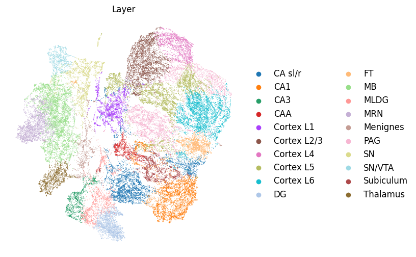
[13]:
sc.pp.neighbors(adata1, use_rep='X_SE', key_added='X_SE')
adata1.obsm['umap_SE'] = sc.tl.umap(adata1, neighbors_key='X_SE', copy=True).obsm['X_umap']
with rc_context({'figure.figsize': (6,6)}):
    sc.pl.embedding(adata1, color='Layer', basis="umap_SE",
                    frameon=False, wspace=0.4, vmax='p99',legend_fontsize=12)
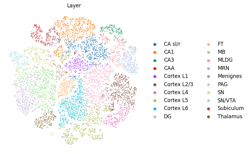
[14]:
adata1.obsm['tsne_SE'] = sc.tl.tsne(adata1, use_rep='X_SE', copy=True).obsm['X_tsne']
with rc_context({'figure.figsize': (6,6)}):
    sc.pl.embedding(adata1, color='Layer', basis="tsne_SE",
                    frameon=False, wspace=0.4, vmax='p99',legend_fontsize=12)
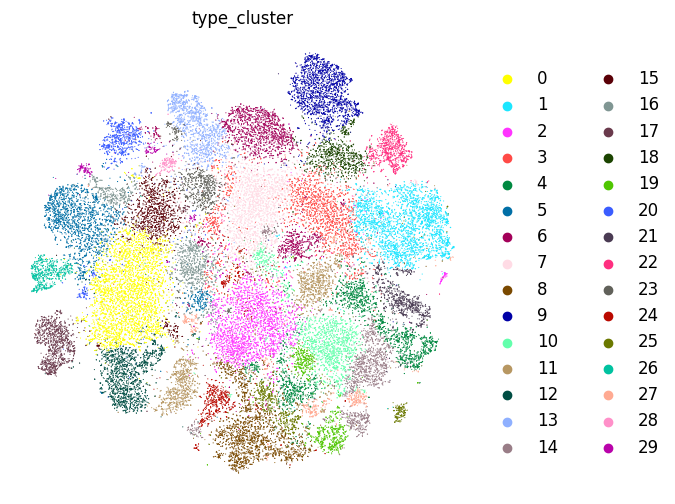
Clustering for CE
[15]:
SECE.cluster_func(adata1, clustering='leiden', use_rep='X_CE', res=1.75, key_add='type_cluster')
with rc_context({'figure.figsize': (6.5,7.5)}):
    sc.pl.embedding(adata1, basis='spatial', color=['type_cluster'],
                    frameon=False, s=9)

[22]:
adata1.obsm['tsne_CE'] = sc.tl.tsne(adata1, use_rep='X_CE', copy=True).obsm['X_tsne']
with rc_context({'figure.figsize': (6,6)}):
    sc.pl.embedding(adata1, color='type_cluster', basis="tsne_CE",
                    frameon=False, wspace=0.4, vmax='p99',legend_fontsize=12)
[16]:
adata1
[16]:
AnnData object with n_obs × n_vars = 50140 × 18575
    obs: 'annotation', 'x', 'y', 'size', 'n_counts', 'layer_cluster', 'Layer', 'type_cluster'
    var: 'n_cells'
    uns: 'log1p', 'layer_cluster_colors', 'Layer_colors', 'X_SE', 'type_cluster', 'leiden', 'type_cluster_colors'
    obsm: 'spatial', 'X_CE', 'X_SE', 'umap_SE', 'tsne_SE'
    layers: 'counts', 'expr'
    obsp: 'X_SE_distances', 'X_SE_connectivities', 'type_cluster_distances', 'type_cluster_connectivities'
[17]:
adata1.write(f'{result_path}/adata1.h5ad')